Modeled reconstruction · 90-frame sequence
Miami-Dade landfall wind field
The animation is centered on the southeast Florida landfall and includes modeled wind decay over land using an approximation of 1926 land use.
 1926HURRICANE.COM
Evidence · Reanalysis · Reconstruction
This page keeps three different kinds of evidence visibly separate: what observers recorded in 1926, what later official reanalysis concluded, and what modern modeling can reconstruct. The distinction matters because a modeled wind field can be scientifically useful without being a direct measurement.
Weather Bureau records, Monthly Weather Review reports, ship and land observations, pressure readings, wind reports and storm-surge evidence created during or immediately after the hurricane.
HURDAT reanalysis, NOAA/HRD evidence ledgers and modern landfall parameters that reassess the historical record using the best available observations and methods.
Modern wind-swath and land-decay products that use the historical/reanalyzed storm parameters plus estimated structural inputs to visualize a plausible wind field.
Science in its time
Before comparing modern reanalysis with modeled wind fields, it helps to understand the observational world Richard Gray and his colleagues actually worked in: ships, surface stations, barometers, telegraph, radio and empirical track knowledge — but no radar, satellites, routine reconnaissance aircraft or numerical hurricane models.
Modern reconstruction · Brian McNoldy / University of Miami
Brian McNoldy’s 1926 products translate the reanalyzed storm into a visual estimate of how the surface wind field may have looked. They are a reconstruction, not a replacement for HURDAT2 or the contemporary observations.
The animation is centered on the southeast Florida landfall and includes modeled wind decay over land using an approximation of 1926 land use.
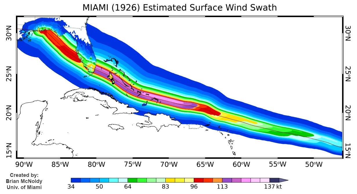
A storm-lifetime estimate of the maximum modeled surface wind experienced along the track.
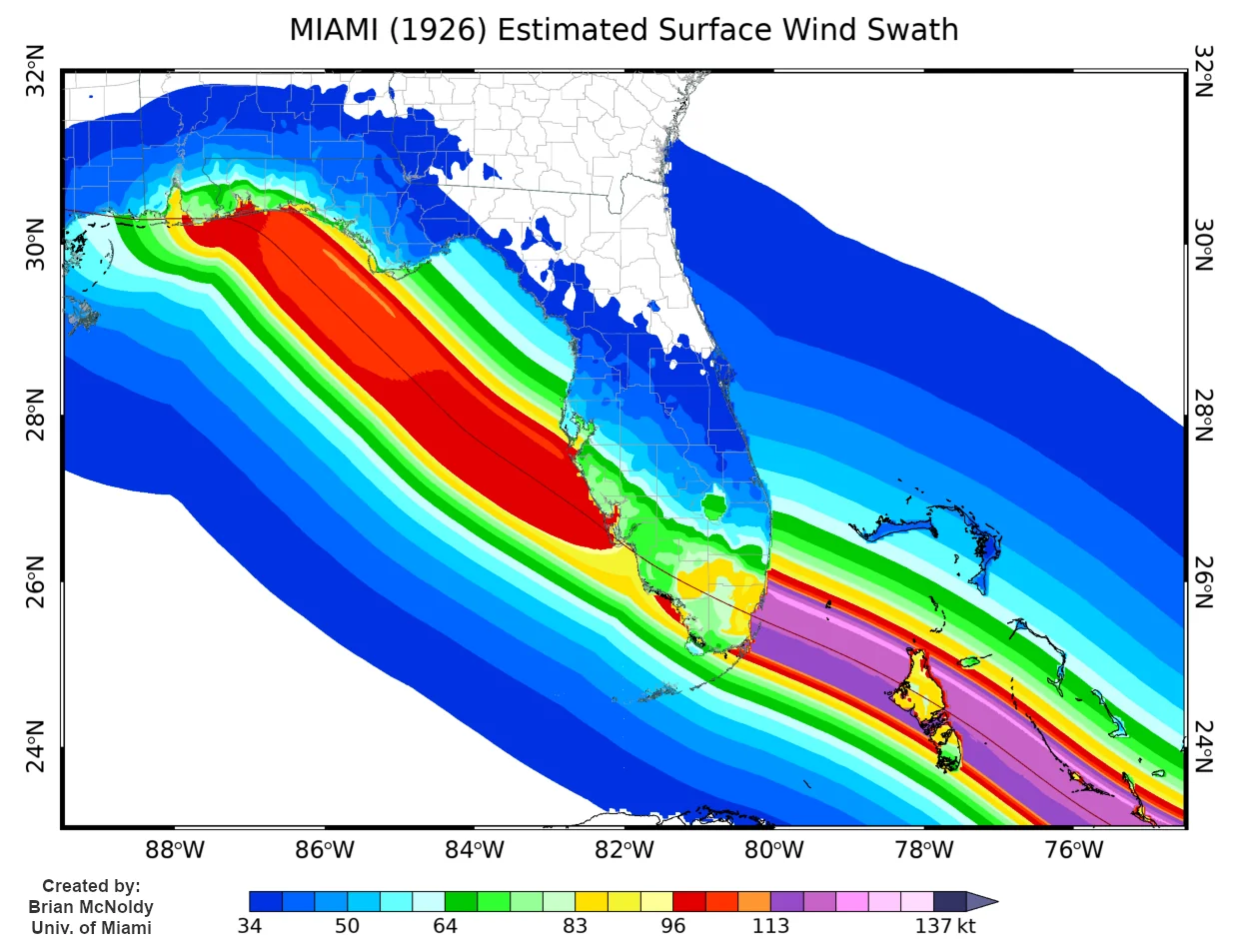
A closer view of the modeled swath over Florida, including the Miami landfall and passage into the Gulf.
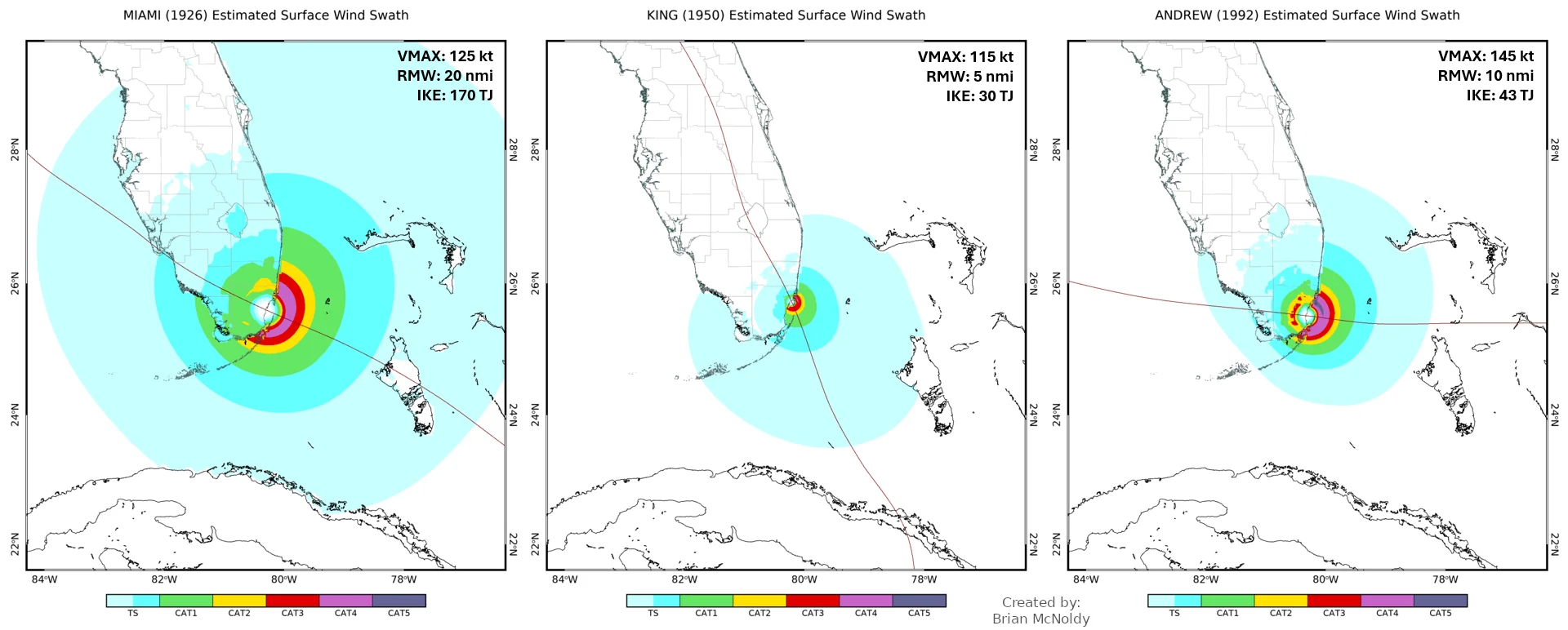
McNoldy’s comparison shows why peak wind alone does not describe a hurricane’s footprint. The 1926 storm had a much broader modeled core and far greater integrated kinetic energy than either King or Andrew, even though Andrew had the highest peak wind.
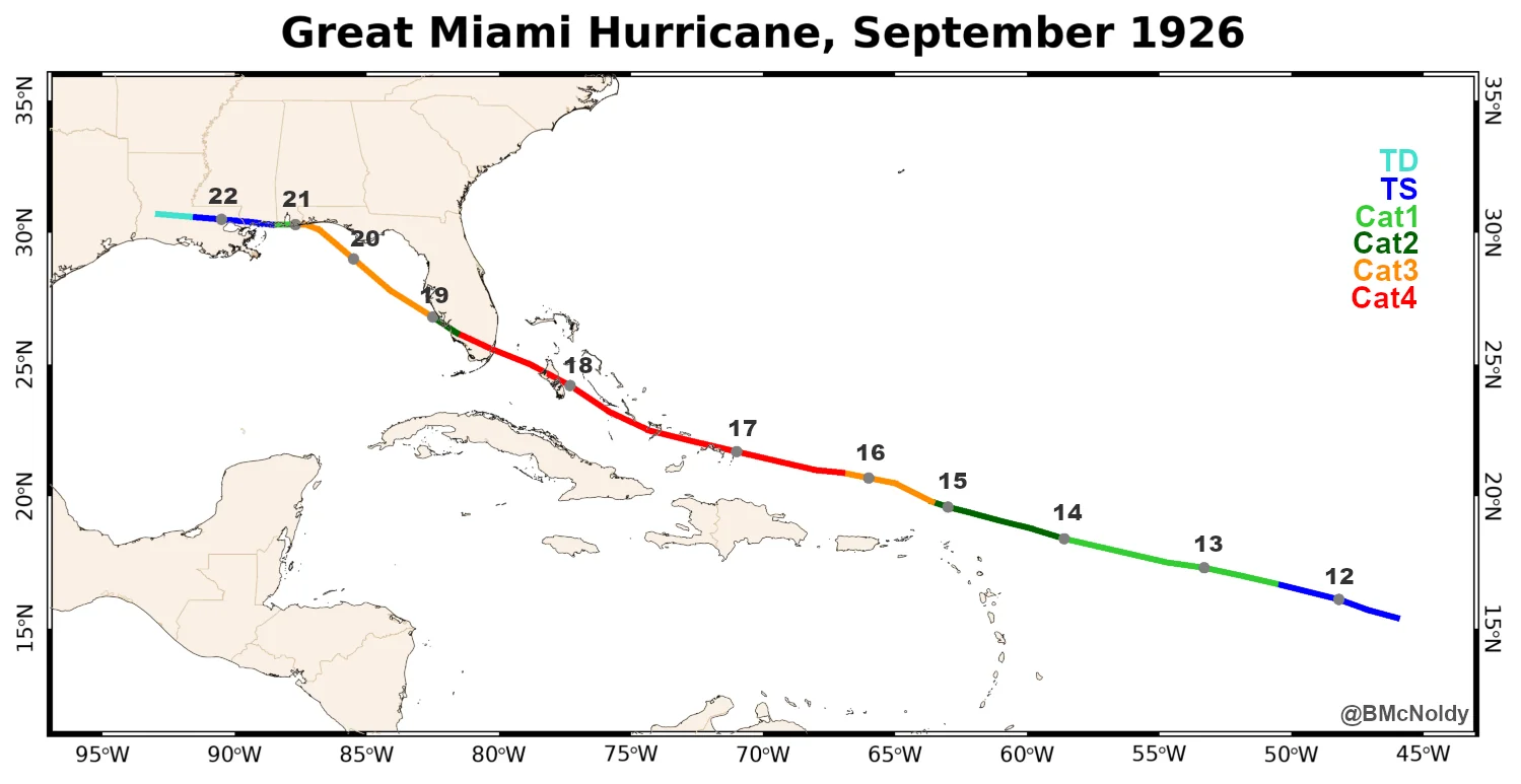
McNoldy’s overview map provides context for the modeled products. The interactive Storm Atlas plots NOAA’s HURDAT2 positions and links each fix to its source data.
Why storm size matters
In McNoldy’s creator-supplied comparison, the 1926 hurricane is modeled with about 145 mph peak wind, an RMW near 23 miles, and 170 TJ of integrated kinetic energy (IKE). King is about 130 mph, RMW 6 miles, and 30 TJ; Andrew is about 165 mph, RMW 12 miles, and 43 TJ.
| Storm | Peak wind | RMW | IKE |
|---|---|---|---|
| Miami 1926 | ~145 mph | ~23 mi | 170 TJ |
| King 1950 | ~130 mph | ~6 mi | 30 TJ |
| Andrew 1992 | ~165 mph | ~12 mi | 43 TJ |
That makes the modeled 1926 IKE roughly 5.7 times King’s and about 4.0 times Andrew’s. Andrew was more intense at the center, but the 1926 hurricane’s much larger wind field carried substantially more total wind energy across South Florida.
What does 170 TJ actually mean?
Integrated kinetic energy (IKE) adds up the kinetic energy contained in the hurricane’s damaging near-surface wind field. It depends on both how fast the wind is blowing and how much area those winds cover. That is why storm size matters so much.
It is not simply the energy inside the radius of maximum wind. The RMW helps define the storm’s inner structure, but the IKE calculation uses the broader modeled or analyzed surface wind field — including the extent of tropical-storm-force, hurricane-force and stronger winds — and sums the kinetic-energy contribution across that circulation.
One terajoule (TJ) is one trillion joules. The number is not meant to be intuitive by itself; its value here is comparative. McNoldy’s reconstruction gives Miami 1926 about 170 TJ, versus 43 TJ for Andrew and 30 TJ for King at their southeast Florida landfalls. In other words, Andrew had the higher peak wind, but the 1926 hurricane placed very strong winds over a much larger area.
The underlying physics is the kinetic-energy relationship ½ρU², where ρ is air density and U is wind speed. For hurricane IKE, that energy density is integrated across the analyzed near-surface storm wind field. Because wind speed is squared, stronger winds contribute disproportionately; because the calculation is integrated over the wind field, a large storm can accumulate far more total energy than a compact storm with a higher maximum wind.
Brian McNoldy’s original graphic retains its creator units (kt and nmi). The museum text converts those values to mph and statute miles to match the site-wide display standard. IKE is shown in terajoules as supplied by the creator.
Credit & use
Graphics and animation reproduced with permission of Brian McNoldy.
Original analysis and methodology ↗Research trail
The records below show the observational, reanalysis and reconstruction sources used to keep the technical interpretation traceable.